An Introduction to Estimating Exponential Random Graph Models for Large Networks with `bigergm` • bigergm

This vignette briefly introduces how to use the R package bigergm, which estimates Hierarchical Exponential-Family Random Graph Models (HERGMs, Schweinberger and Handcock 2015). The package bigergm builds on the R packages lighthergm (Martínez Dahbura et al. 2021) and hergm (Schweinberger and Luna 2018) and applies scalable algorithms to scale the estimation up to big networks with up to 50 K population members (see Martínez Dahbura et al. (2021) and Fritz et al. (2024)).

Exponential Random Graph Models for Large Networks

Exponential Random Graph Models (ERGMs) are a popular class of models for network data. They model the probability of observing a network as a function of network statistics, such as the number of edges and triangles. ERGMs are commonly employed in social network analysis but have some limitations when applied to large networks. The main limitation is that the likelihood function is intractable for large networks, making it difficult to estimate the model parameters. At the same time, larger networks warrant more complex models to capture the underlying structure of the network.

To address these limitations, bigergm implements a scalable algorithm for estimating HERGMs, which generalize ERGMs that allow for local dependence induced by non-overlapping blocks of nodes with network data. Introduced by Schweinberger and Handcock (2015), complex dependence is allowed only between nodes within the same block. Thereby, we obtain a more flexible model that can capture the cohesive subgroups in the network globally while accounting for dependence within these subgroups on the local level.

Model Specification

Consider a network of $N$ population members encompassed in the set $\mathcal{P} = \{1, \ldots, N\}$ . Define the adjacency matrix corresponding to this network as $\mathbf{Y}= (Y_{i,j}) \in \mathbb{R}^{N\times N}$ , where $Y_{i,j}$ is the entry in the $i$ -th row and $j$ -th column of the matrix. If $Y_{i,j} = 1$ , nodes $i$ and $j$ are connected; otherwise, they are not connected. In this vignette we only regard undirected networks, thus the adjacency matrix is symmetric, i.e., $Y_{i,j} = Y_{j, i}$ .
Note, however, that the package bigergm also supports directed networks. The number of blocks is denoted as $K$ and $\mathbf{z}= (z_{i,k}) \in \mathbb{R}^{N\times K}$ is the block membership matrix with entries $z_{i,k}$ equal to 1 if node $i$ belongs to block $k$ and 0 otherwise. Let $\mathbf{Y}_{k,l}$ be the submatrix of $\mathbf{Y}$ of the connections between blocks $k$ and $l$ , i.e., the matrix including the connections between population members $i$ and $j \in \mathcal{P}$ with $z_{i,k} = z_{j,l}= 1$ . The submatrix $\mathbf{Y}_{k,k}$ of $\mathbf{Y}$ contains the connections within block $k$ , i.e., the matrix including the connections between population members $i$ and $j \in \mathcal{P}$ with $z_{i,k} = z_{j,k}= 1$ . Let $\mathbf{x} = (x_{i,p}) \in \mathbb{R}^{N\times p}$ be a matrix of nodal covariates, where $p$ is the number of covariates and $x_{i,p}$ refers to the $p$ th nodal covariate of population member $i$ . For the context of bigergm, assume that all nodal covariates are categorical. Generally, we refer to random variables by capitalized letters and their realizations by lowercase letters.

Given this notation, the probability of observing the network $\mathbf{Y}$ for a given the block membership matrix $\mathbf{Z}$ is given by: $\mathbf{P}_\theta(\mathbf{Y} = \mathbf{y} | \mathbf{Z} = \mathbf{z},\mathbf{X} = \mathbf{x}) = \prod_{k \neq l} \mathbf{P}_{\alpha}(\mathbf{Y}_{k,l} | \mathbf{Z} = \mathbf{z}, \mathbf{X} = \mathbf{x}) \prod_{k} \mathbf{P}_{\beta}(\mathbf{Y}_{k,k} | \mathbf{Z} = \mathbf{z}, \mathbf{X} = \mathbf{x}),$ where $\mathbf{P}_{\alpha}(\mathbf{Y}_{k,l} | \mathbf{Z} = \mathbf{z})$ is the probability of observing the edges between blocks $k$ and $l$ given $\mathbf{z}$ and $\mathbf{P}_{\beta}(\mathbf{Y}_{k,k} | \mathbf{Z} = \mathbf{z})$ is the probability of observing the edges within block $k$ given $\mathbf{z}$ . The parameter vectors $\alpha$ and $\beta$ are the coefficients of the between-block and within-block networks, respectively. How these two models are specified is sketched in the next two paragraphs.

Between-block Model

For the probability model for edges between population members of blocks $k$ and $l$ , we employ a network model assuming dyadic independence between the edges:

$\mathbf{P}_{\alpha}(\mathbf{Y}_{k,l} = \mathbf{y}_{k,l} | \mathbf{Z} = \mathbf{z}, \mathbf{X} = \mathbf{x}) = \prod_{(i,j) \text{; } z_{ik} = 1 \text{, } z_{jl} = 1} \mathbf{P}_{\alpha}(Y_{i,j} = y_{i,j} | \mathbf{Z} = \mathbf{z}, \mathbf{X} = \mathbf{x}),$ where $\mathbf{P}_{\alpha}(Y_{i,j} = y_{i,j} | \mathbf{Z} = \mathbf{z}, \mathbf{X} = \mathbf{x}) = (\pi_{k,l}(\alpha, \mathbf{x}))^{y_{i,j}} (1 - \pi_{k,l}(\alpha, \mathbf{x}))^{1 - y_{i,j}}$ is the probability distribution of a Bernoulli distribution with parameter $\pi_{k,l}(\alpha, \mathbf{x})$ evaluated at $y_{i,j}$ .
The parameter $\pi_{k,l}(\alpha, \mathbf{x})$ is the probability of observing an edge between nodes $i$ and $j$ with $z_{i,k} = z_{j,l} = 1$ and have different forms:

For the standard Stochastic Block Model (SBM), the probability of observing an edge between nodes $i$ and $j$ is given by $\alpha_{k,l}$ .
Extending this simplistic model, the current implementation allows the usage of nodematch statistics to include the nodal covariates $\mathbf x$ in the model, implying the following probability for $y_{i,j}$ with $z_{i,k} = z_{j,l} = 1$ :

$\pi_{k,l}(\alpha, \mathbf{x}) = \text{logit}^{-1}\left(\alpha + \sum_{p = 1}^P \alpha_p \, \mathbb{I}\left(x_{i,p} = x_{j,p}\right) \right),$ where all parameters ( $\alpha$ and $\alpha_p$ for $p = 1, \ldots, P$ ) can vary for each pair of blocks $k$ and $l$ .

Within-block Model

The probability of observing the edges within block $k$ is modeled as a function of network statistics, such as the number of edges or triangles within block $k$ . We specify the within-block networks as exponential-family random graph models: $\mathbf{P}_{\beta}(\mathbf{Y}_{k,k} = \mathbf{y}_{k,k} | \mathbf{Z} = \mathbf{z}, \mathbf{X} = \mathbf{x}) = \exp\left(\beta^\top \mathbf{s}(\mathbf{y}_{k,k}, \mathbf{x})\right)/ c(\beta, \mathbf{z}, \mathbf{x}),$ where $\mathbf{s}(\mathbf{y}_{k,k}, \mathbf{x})$ is a vector of sufficient statistics counting, e.g., the edges within block $k$ and $c(\beta, \mathbf{z}, \mathbf{x})$ is a normalizing constant guaranteeing that the probability distribution sums to one. Examples of network statistics include the number of edges, triangles, and degree statistics (see Morris, Handcock, and Hunter (2008) and all references therein).

Estimation

Since the block membership matrix $\mathbf{z}$ is usually unobserved, we estimate it. Therefore, we assume that the now random block membership matrix $\mathbf{Z}$ is a latent variable and following a multinomial distribution: $\mathbf{Z} \sim \text{Multinomial}(1; \gamma_1, \ldots, \gamma_K),$ where $\gamma_k$ is the marginal probability that a node belongs to block $k$ for $k = 1, \ldots, K$ . Given this context, the model is estimated in two steps by the algorithm proposed by Babkin, Stewart, and Schweinberger (2020):

Recover the block membership matrix $\mathbf{Z}$ by maximizing a lower bound of the likelihood from the observed network $\mathbf{Y}$ (see Babkin, Stewart, and Schweinberger (2020) and Vu, Hunter, and Schweinberger (2013) for details).
Given the estimated block membership matrix $\hat{\mathbf{Z}}$ , estimate the coefficients $\alpha$ and $\beta$ by maximizing the pseudo-likelihood of the observed network $\mathbf{Y}$ . The pseudo-likelihood of the observed network $\mathbf{Y}$ given the estimated block membership matrix $\hat{\mathbf{Z}}$ is equivalent to the likelihood of a logistic regression model and can, therefore, be estimated by standard optimization algorithms. For this step, the entire computational machinery implemented in the ergm package is used.

However, note that the first step is unnecessary if the block membership matrix is known.

The package bigergm implements a scalable algorithm for estimating HERGMs even for large networks by exploiting the structure of the model and the network data (details are provided in Martínez Dahbura et al. (2021) and Fritz et al. (2024)).

Installation

You can install the CRAN version of bigergm by running the following command:

install.packages("bigergm")

A simple example

Let’s start with a simple example using the toy network included in the package. The toy network is a small network with a clear community structure, which is helpful for testing the package.

# Load the network object.
data(toyNet)
# Plot the network.
plot(toyNet, vertex.col = rep(c("tomato", "steelblue", "darkgreen", "black"),
                        each = toyNet$gal$n/4))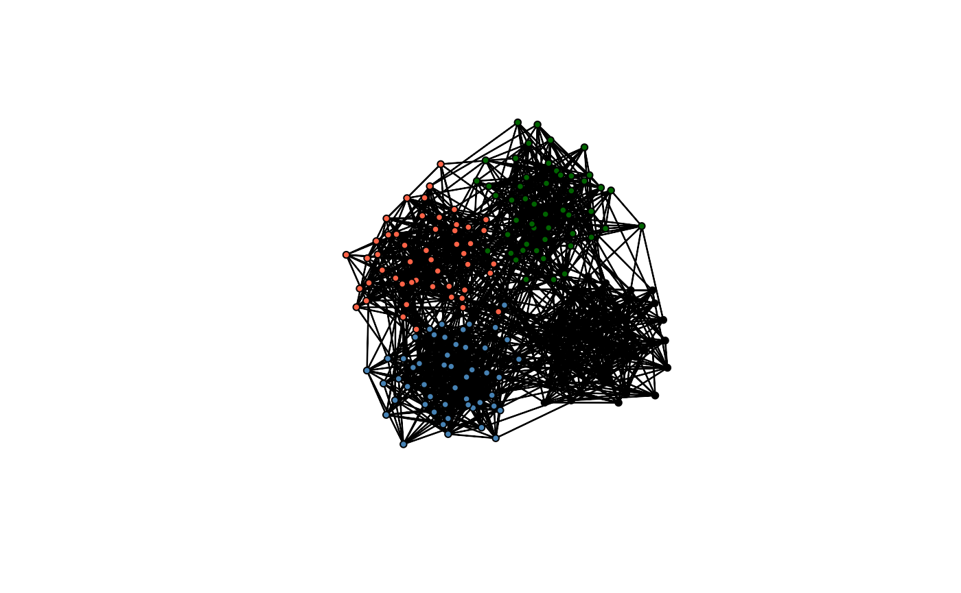

It is visible that this network has a cluster or community structure. Although this is an artificial network, we often observe such community structures in real-world social networks. Exploiting this stylized fact, we model the way population members in a network get connected differently for connections across and within communities:

Connections across communities happen by luck, influenced by homophily
Connections within communities also consider interdependencies among links. For example, the probability that population members $i$ and $j$ get connected may be influenced by a third population member $k$ .

To estimate an Exponential Random Graph model with local dependence, we first need to specify the model formula that specifies the model. As described in the previous section, the model consists of two parts: the between-block model and the within-block model. To ease this step, both parts are specified in one formula very similar to specifying a model in ergm::ergm(). All terms that induce dependence are excluded from the between block model, while the within block model includes all terms. In the following example, we include the number of edges, the number of triangles, and nodematch statistics for the nodal covariates x and y in the model.

model_formula <- toyNet ~ edges + nodematch("x") + nodematch("y") + triangle

Assuming that covariate ‘x’ is the first and covariate ‘y’ is the second covariate, the probability of observing $Y_{i,j}$ with $z_{i,k} = z_{j,l} = 1$ is specified by: $\pi_{k,l}(\alpha, \mathbf{x}) = \text{logit}^{-1}\left(\alpha_0 + \alpha_{2}\, \mathbb{I}(x_{i,1} = x_{j,1}) + \alpha_2\, \mathbb{I}(x_{i,2} = x_{j,2})\right)$ and the sufficient statistics of the within-block model are: $\mathbf{s}(\mathbf{y}_{k,k}, \mathbf{x}) = \left(\sum_{i<j} y_{i,j}, \sum_{i<j} \mathbb{I}(x_{1,i} = x_{1,j})\, y_{i,j}, \sum_{i<j} \mathbb{I}(x_{1,i} = x_{1,j})\, y_{i,j}, \sum_{i<j}\sum_{h \neq i,j} y_{i,j}\, y_{i,h}\, y_{h,j}\right).$

We can estimate the specified model with the bigergm() function, which takes the following parameters:

object: A formula specifying the model to estimate (as detailed in the previous paragraph). See help(bigergm) for how providing a fitted bigergm object can be used to continue the estimation.
clustering_with_features: boolean value set to TRUE, if the algorithm should consider nodal covariates in the first step of the estimation.
n_blocks: Number of blocks to recover (in the above explanations, $K$ ).
n_MM_step_max: Maximum number of MM algorithm steps.
tol_MM_step: Threshhold when convergence is reached. Following Vu, Hunter, and Schweinberger (2013), we stop the algorithm when the relative change in the lower bound of the objective function is less than tol_MM_step.
estimate_parameters: boolean value set to TRUE, if the algorithm should estimate the parameters after the block recovery step.
check_block_membership: boolean value set to TRUE, if the algorithm should keep track of block memberships at each MM iteration.

There are other parameters that you can specify, which are detailed in the documentation (see help(bigergm)).

res <-bigergm(
    # The model you would like to estimate
    object = model_formula,
    # The number of blocks
    n_blocks =  4, 
    # The maximum number of MM algorithm steps
    n_MM_step_max = 100,
    # The tolarence for the MM algorithm
    tol_MM_step = 1e-6,
    # Perform parameter estimation after the block recovery step
    estimate_parameters = TRUE,
    # Indicate that clustering must take into account nodematch on characteristics
    clustering_with_features = TRUE,
    # Keep track of block memberships at each EM iteration
    check_block_membership = TRUE, 
    # Name the heuristic algorithm used for initializing the block memberships
    initialization = "walktrap"
)

We can plot the estimated the objective function of the first estimation step recovering the latent community structure over iterations. This allows us to check whether this step has converged.

plot(1:length(res$MM_lower_bound),
     res$MM_lower_bound, type = "l", xlab = "Iterations", ylab = "Lower Bound")

The result indicates that the clustering step converged at the early stage. Note that the number of iterations you need to perform (n_MM_step_max) varies depending on the network’s size and clarity in community structure. The convergence of the lower bound does, however, not guarantee the convergence of the clustering step to a unique maximizer. Therefore, restarting the algorithm with different initializations may be advisable in practice.

You can check the clustering result by plotting the network with nodes colored by the estimated block membership. The edges are grey if the two population members are from different blocks and black otherwise.

plot(res)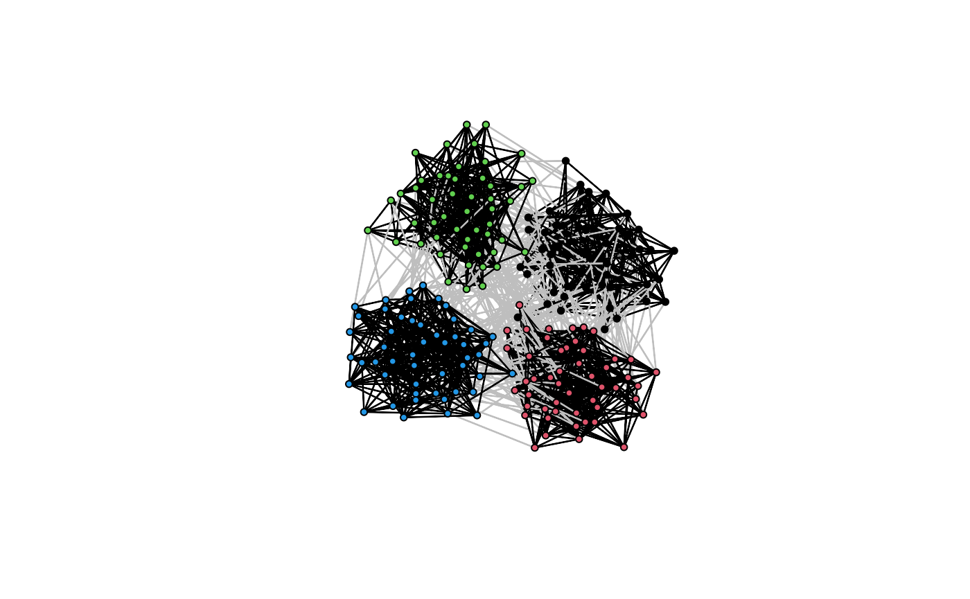

The parameter estimates of $\alpha$ and $\beta$ may be inspected using the summary() function.

# For the between networks
summary(res$est_between)
#>  Results:
#> 
#>             Estimate Std. Error MCMC % z value Pr(>|z|)    
#> edges       -4.21749    0.07482      0 -56.369   <1e-04 ***
#> nodematch.x  0.78273    0.16144      0   4.848   <1e-04 ***
#> nodematch.y  0.38854    0.18433      0   2.108    0.035 *  
#> ---
#> Signif. codes:  0 '***' 0.001 '**' 0.01 '*' 0.05 '.' 0.1 ' ' 1
#> 
#> Warning:  The standard errors are based on naive pseudolikelihood and are suspect. Set control.ergm$MPLE.covariance.method='Godambe' for a simulation-based approximation of the standard errors.
#> 
#>      Null Pseudo-deviance: 2576  on 8  degrees of freedom
#>  Residual Pseudo-deviance: 2551  on 5  degrees of freedom
#>  
#> AIC: 2557  BIC: 2558  (Smaller is better. MC Std. Err. = NA)

# For the within networks
summary(res$est_within)
#> Call:
#> ergm::ergm(formula = within_formula, offset.coef = offset.coef, 
#>     estimate = method, control = control)
#> 
#> Maximum Pseudolikelihood Results:
#> 
#>             Estimate Std. Error MCMC % z value Pr(>|z|)    
#> edges       -1.80056    0.06660      0 -27.036   <1e-04 ***
#> nodematch.x  0.86683    0.10351      0   8.375   <1e-04 ***
#> nodematch.y  0.96478    0.10368      0   9.305   <1e-04 ***
#> triangle     0.14615    0.01744      0   8.382   <1e-04 ***
#> ---
#> Signif. codes:  0 '***' 0.001 '**' 0.01 '*' 0.05 '.' 0.1 ' ' 1
#> 
#> Warning:  The standard errors are based on naive pseudolikelihood and are suspect. Set control.ergm$MPLE.covariance.method='Godambe' for a simulation-based approximation of the standard errors.
#> 
#>      Null Pseudo-deviance: 6793  on 4900  degrees of freedom
#>  Residual Pseudo-deviance: 5154  on 4896  degrees of freedom
#>  
#> AIC: 5162  BIC: 5188  (Smaller is better. MC Std. Err. = 0)

Currently, only nodematch() terms are supported as a way to include covariates in the model.

Simulation

You can simulate networks with local dependence by using bigergm () and simulate_bigergm() functions. The simulate.bigergm() function is a wrapper around the simulate_bigergm() function for a particular fitted bigergm object. To apply the simulate.bigergm() function, you only need to provide the fitted bigergm object.

simulate(res, seed = 1)
#>  Network attributes:
#>   vertices = 200 
#>   directed = FALSE 
#>   hyper = FALSE 
#>   loops = FALSE 
#>   multiple = FALSE 
#>   bipartite = FALSE 
#>   total edges= 1464 
#>     missing edges= 0 
#>     non-missing edges= 1464 
#> 
#>  Vertex attribute names: 
#>     block vertex.names x y 
#> 
#>  Edge attribute names not shown

The simulate_bigergm() function allows you to simulate networks with local dependence from scratch. The function requires coefficients for the between and within connections, the formula for the model, the number of simulations to return, and the output format. Depending on the output format, the function returns a list with the network statistics for the between and within connections, the adjacency matrix of the simulated network, or the network object itself.

sim_net <- bigergm::simulate_bigergm(
  formula = model_formula,
  # The coefficients for the between connections
  coef_between = res$est_between$coefficients,
   # The coefficients for the within connections
  coef_within = res$est_within$coefficients,
  # Number of simulations to return
  nsim = 1,
  # If `stats` a list with network statistics 
  # for the between and within connections is returned
  output = "network"
)

After simulating the network, you can plot it to assess whether the community structure is preserved.

plot(sim_net)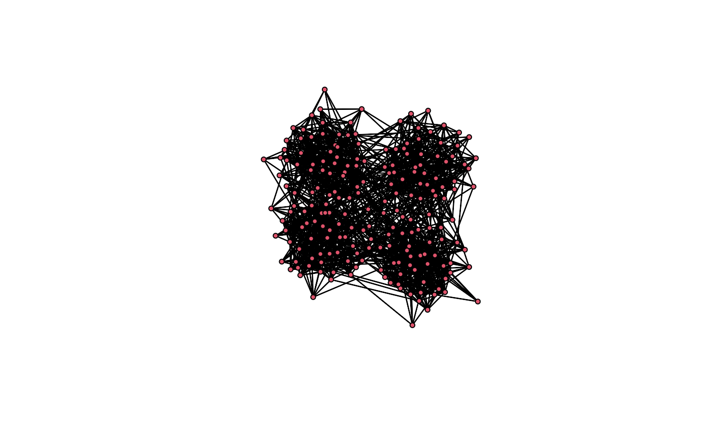

Goodness-of-fit

Following the estimation, consider evaluating the goodness-of-fit of the model. In line with the ERGM literature, we provide a goodness-of-fit assessment that evaluates how good simulations from the model fit the observed network. We provide a function gof() to carry out this task:

gof_res <- gof(
  # The object returned by bigergm::bigergm()
  object = res,
  # The number of simulations to use
  nsim = 100, 
  # Compute the geodesic distance for the observed and each simulated network
  compute_geodesic_distance = TRUE,
  # Set a seed for reproducibility
  seed = 1234,
  # Start at the observed network
  start_from_observed = TRUE, type = "within",
  # The control parameters for the simulation
  control_within = ergm::control.simulate.formula(MCMC.burnin = 1000, MCMC.interval = 1000)
)

The parameter control_within is used to control the MCMC simulation carried out to simulate from the model. For details we refer to help(ergm::control.simulate.formula). The function evaluates the following metrics for a hundred simulated and observed networks:

network statistics used in the fit or formula provided,
normalized network statistics (the network statistics normalized around the observed statistics),
degree distribution,
geodesic distance, and
edgewise shared partners.

The function bigergm::gof_bigergm() returns a list of data frames for these matrices, allowing you to create plots that match your needs flexibly. Below is an example plot for the degree distribution on the log scale.

degree_gof <- 
  gof_res$simulated$degree_dist %>%
  dplyr::group_by(degree) %>%
  dplyr::summarise(log_mean_share = mean(log(share)),
                   log_sd_share = sd(log(share))) %>%
  dplyr::ungroup()
plot(degree_gof$degree, degree_gof$log_mean_share,
     xlab = "Degree", ylab = "Log Prop. of Nodes",
     ylim = c(-5.5,-1.8), xlim = c(6,17), type = "l", lty = 2)
lines(degree_gof$degree, degree_gof$log_mean_share+ 1.96 * degree_gof$log_sd_share, type = "l", lty = 2)
lines(degree_gof$degree, degree_gof$log_mean_share- 1.96 * degree_gof$log_sd_share, type = "l", lty = 2)
tmp_info <- gof_res$original$degree_dist %>% 
  dplyr::filter(share > 0 & degree < 22)
lines(tmp_info$degree, log(tmp_info$share), lty = 1)

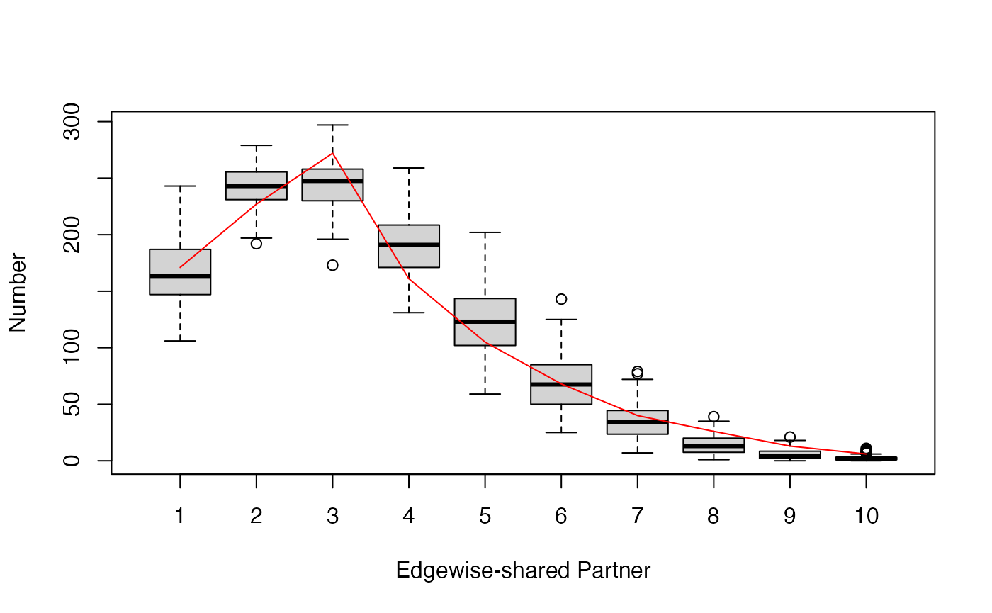
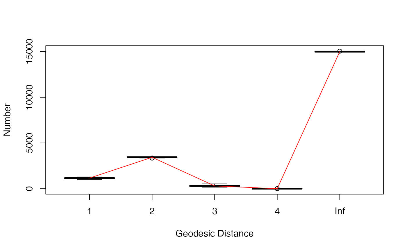
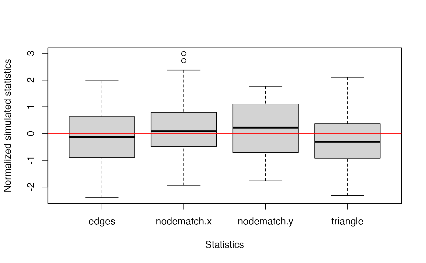
Alternatively, you can use the plot() function to visualize the goodness-of-fit results. Three plots are generated checking whether the estimated model can adequately capture the degree distribution, edgewise-shared partner distribution, and geodesic distances of the observed network. In a fourth plot, the simulated network statistics are plotted normalized around the observed statistics. For a good fit, all values should be around zero. In all plots, the red line represents the observed network, and the boxplot represents the simulated networks.

plot(gof_res)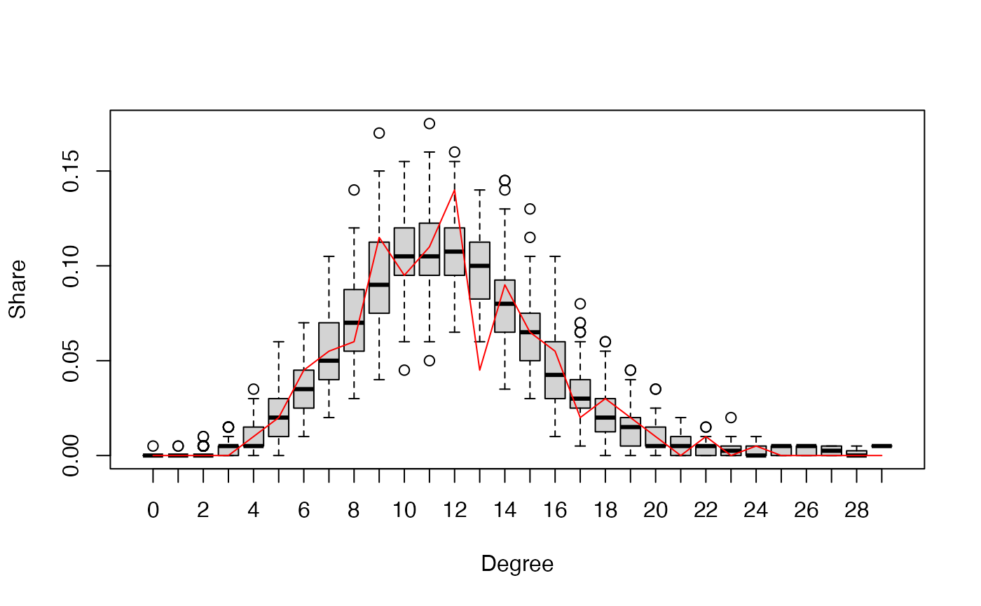

When you work with large networks

If you would like to estimate an bigergm with a large network (say, when the number of nodes $\geq$ 50,000):

Select features sparse enough to fit into memory. Covariates such as gender or race will be too dense to construct feature matrices. This is a non-negligible limitation of our algorithm and will be solved in the future.
Use Python’s infomap to initialize clusters. This is because it is much faster to implement cluster initialization than R functions such as igraph::cluster_infomap(). Set use_infomap_python = TRUE in bigergm::bigergm().
When the MM estimation does not seem to have converged by inspecting the lower bound plot, you can further continue iterating by passing the bigergm class object to bigergm::bigergm() as follows (all parameters such as the number of MM iterations will be inherited from the previous estimation unless specified).
You can also set the parameter only_use_preprocessed = TRUE, if you do not want to preprocess it again and start the estimation again from a different initial value.

res_second <-
  bigergm::bigergm(object = res)

References

Babkin, Sergii, Jonathan Stewart, and Michael Schweinberger. 2020. “Large-Scale Estimation of Random Graph Models with Local Dependence.” Computational Statistics & Data Analysis 152: 107029.

Fritz, Cornelius, Co-Piere Georg, Angelo Mele, and Michael Schweinberger. 2024. “A Strategic Model of Software Dependency Networks,” Working Paper. Available at https://arxiv.org/abs/2402.13375.

Martínez Dahbura, Juan Nelson, Shota Komatsu, Takanori Nishida, and Angelo Mele. 2021. “A Structural Model of Business Card Exchange Networks,” Working Paper. Available at https://arxiv.org/abs/2105.12704.

Morris, Martina, Mark S Handcock, and Dave Hunter. 2008. “Specification of Exponential-Family Random Graph Models: Terms and Computational Aspects.” Journal of Statistical Software 24 (4).

Schweinberger, Michael, and Mark S Handcock. 2015. “Local Dependence in Random Graph Models: Characterization, Properties and Statistical Inference.” Journal of the Royal Statistical Society B 77 (3): 647–76.

Schweinberger, Michael, and Pamela Luna. 2018. “Hergm: Hierarchical Exponential-Family Random Graph Models.” Journal of Statistical Software 85 (1): 1–39.

Vu, Duy, David Hunter, and Michael Schweinberger. 2013. “Model-Based Clustering of Large Networks.” The Annals of Applied Statistics 7 (2): 1010–39.