bigergm: Fit, Simulate, and Diagnose Hierarchical Exponential-Family Models for Big Networks
Roadmap: bigergm workshop
- Local dependence leveraging additional structure
- Preparation and Background
- Demonstration of
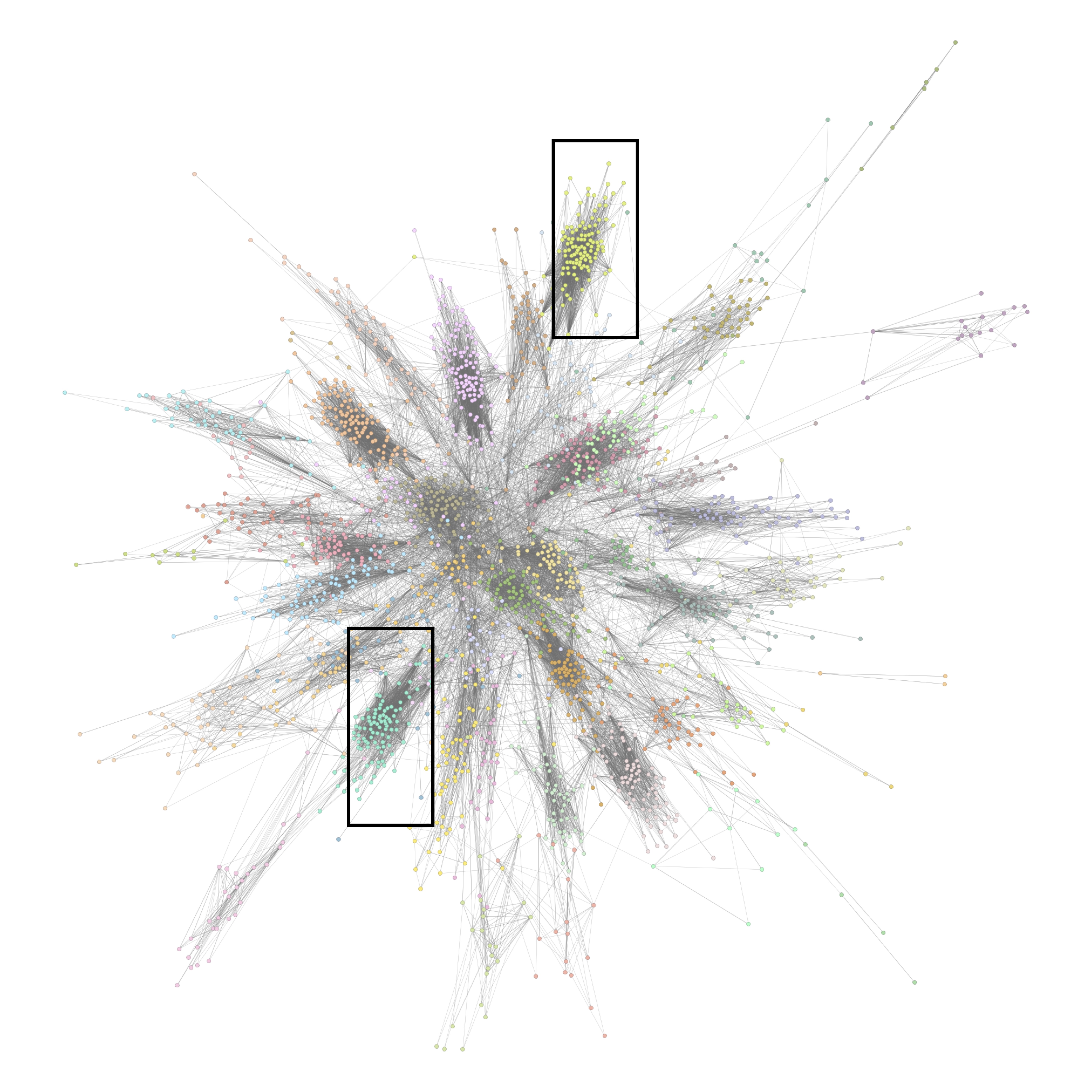
bigergm - Application to Twitter (X): Following Network of State Legislators

Exponential Random Graph Models for Big Networks
Specification: Within-block Model
\[ \mathbb{P}_{W}(\mathbf{x}_{k,k} | \mathbf{y}, \mathbf{z}) = \exp\left(\alpha^\top \mathbf{s}_W(\mathbf{x}_{k,k}, \mathbf{y})\right)/ c_W(\alpha, \mathbf{y}, \mathbf{z}), \]
where
- \(\mathbf{s}_W(\mathbf{x}_{k,k}, \mathbf{y})\) is a vector of network features counting, e.g., the edges within block \(k\)
- \(\alpha\) parameter to estimate
- \(c_W(\alpha, \mathbf{y}, \mathbf{z})\) is the normalizing constant


Estimation
The package bigergm
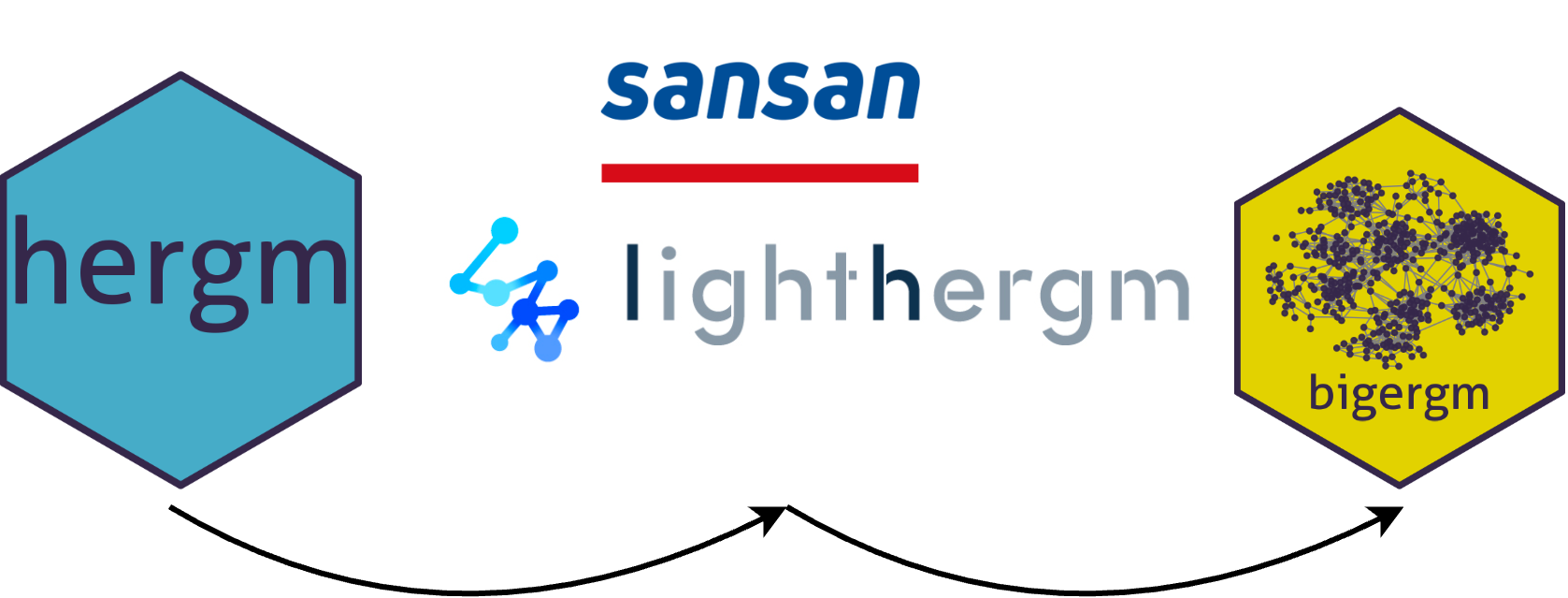
- \(\mathtt{hergm}\): First package developed by Schweinberger & Luna (2018).
- \(\mathtt{lighthergm}\): Scaling up estimation to big networks based on Babkin, Stewart, Long, & Schweinberger (2020) and Dahbura, Komatsu, Nishida, & Mele (2021)
- \(\mathtt{bigergm}\): Extension to directed networks with a clean interface and additional features based on Fritz, Georg, Mele, & Schweinberger (2024)
Installation
- The package can be installed in R as follows:
- An alternative is to install the package from GitHub:

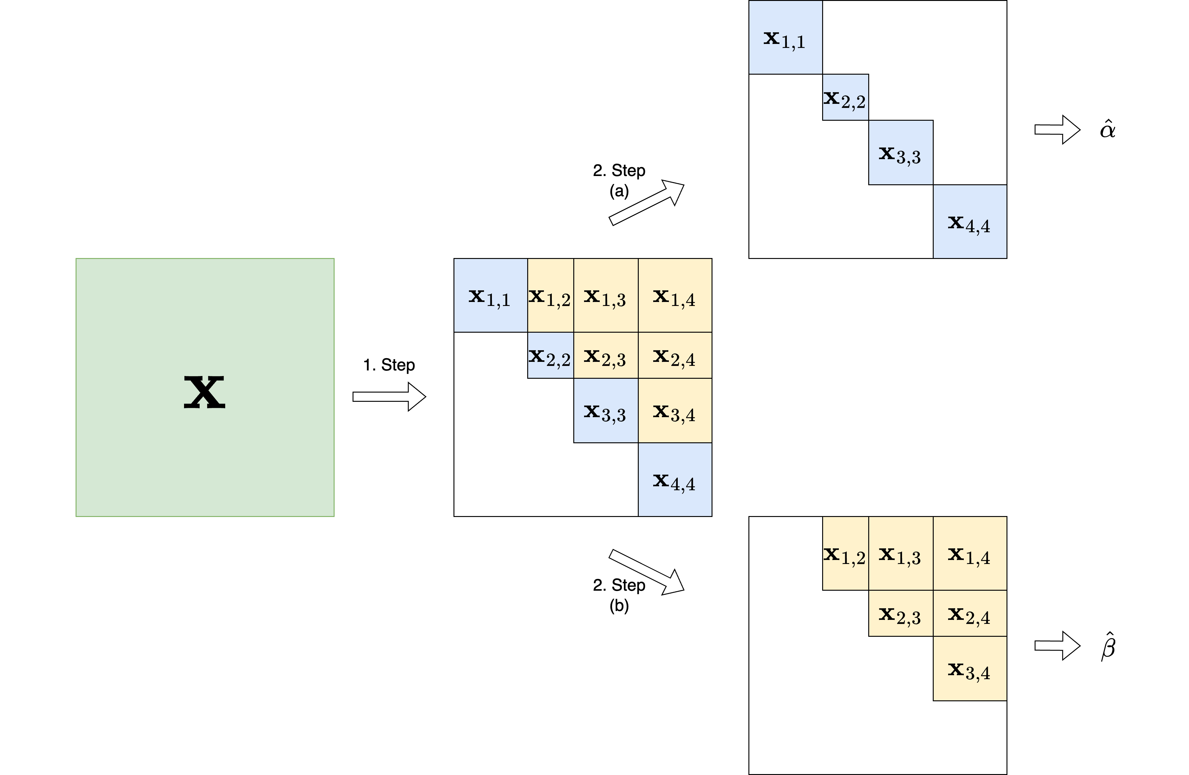
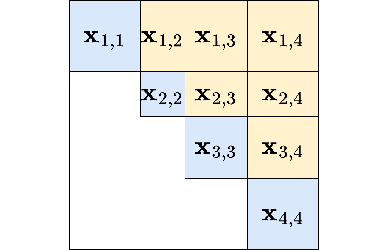
Specify a ERGM with additional structure
- Within-block ERGM (colored blue)
- Between-block ERGM colored yellow)
Simulate
- Plot simulated network

Estimate with unknown block structure

Estimate with unknown block structuree
- Compare the estimated block structure with the true block structure by the adjusted Rand index (ARI)
- Check the clustering step for convergence

Diagnose

Data: Twitter (X) network of U.S. state legislators

1. Specify
- Issue with blocks of different size: Parameters of within-block model may change between blocks
- Solution based on
ergm.multi: Size-dependent parametrizations
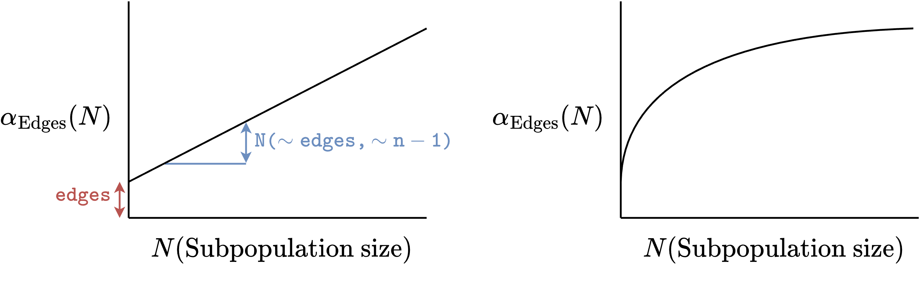
1. Specify
- Issue with blocks of different size: Parameters of the within-block model might change between blocks
- Solution based on
ergm.multi: Size-dependent parametrizations!
2. Estimate
- Exploit that
est_withinis anergmobject - Check if the MCMC chains used for estimation have converged
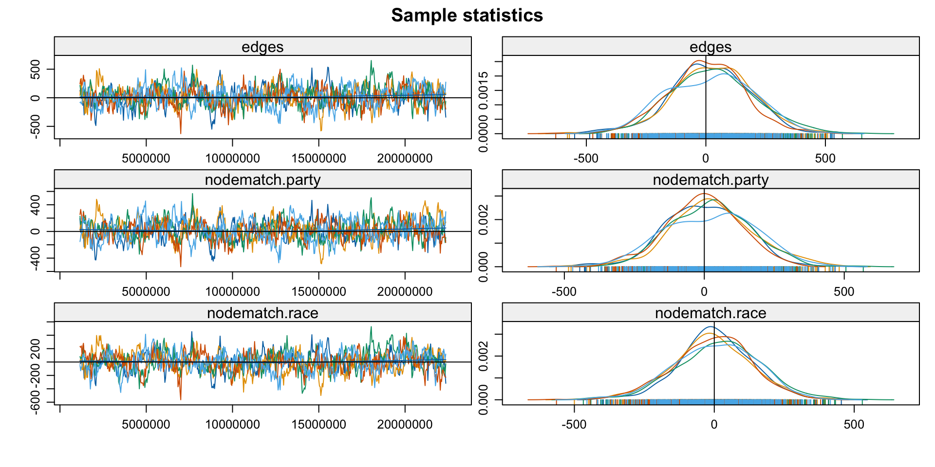
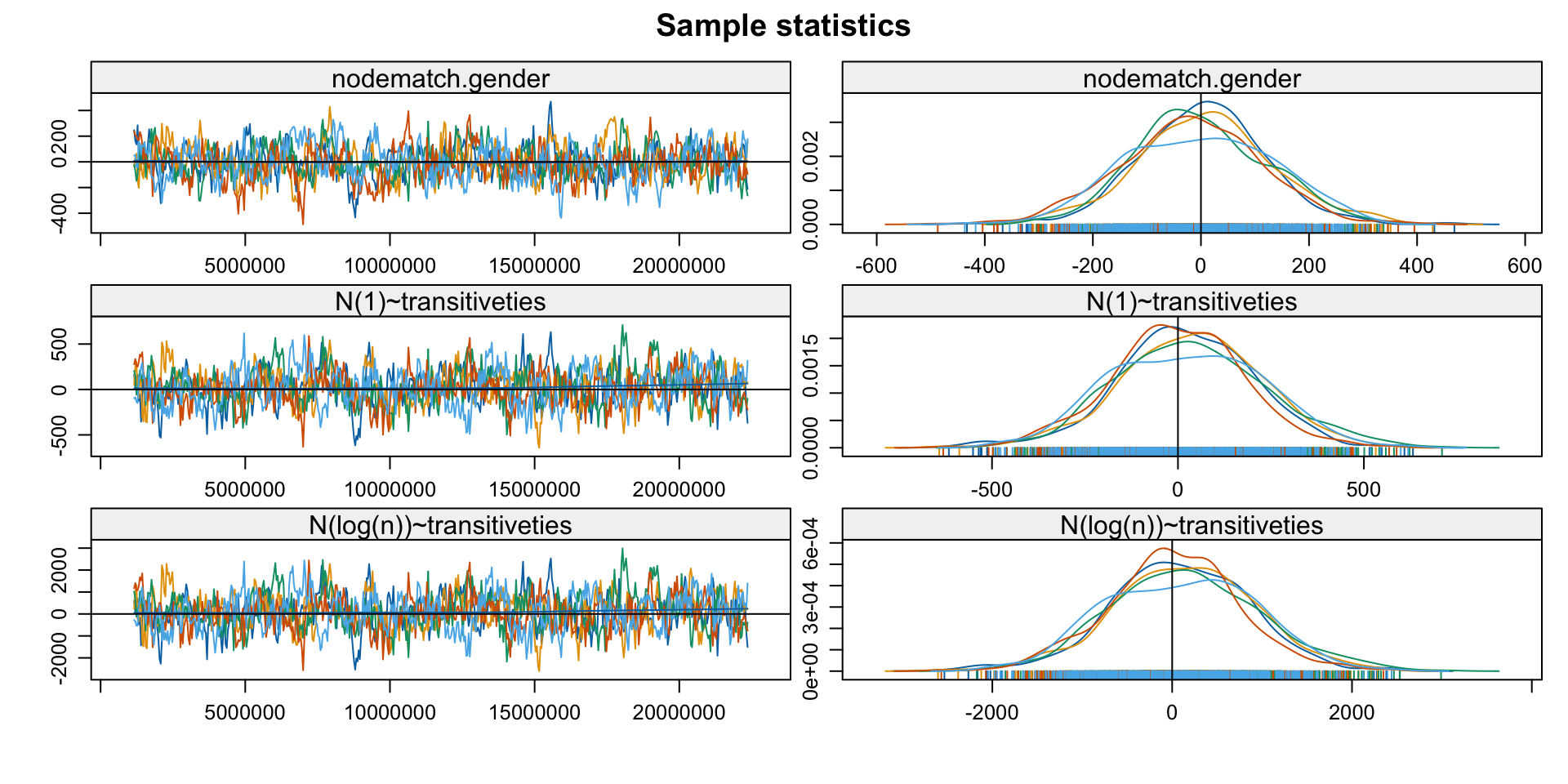
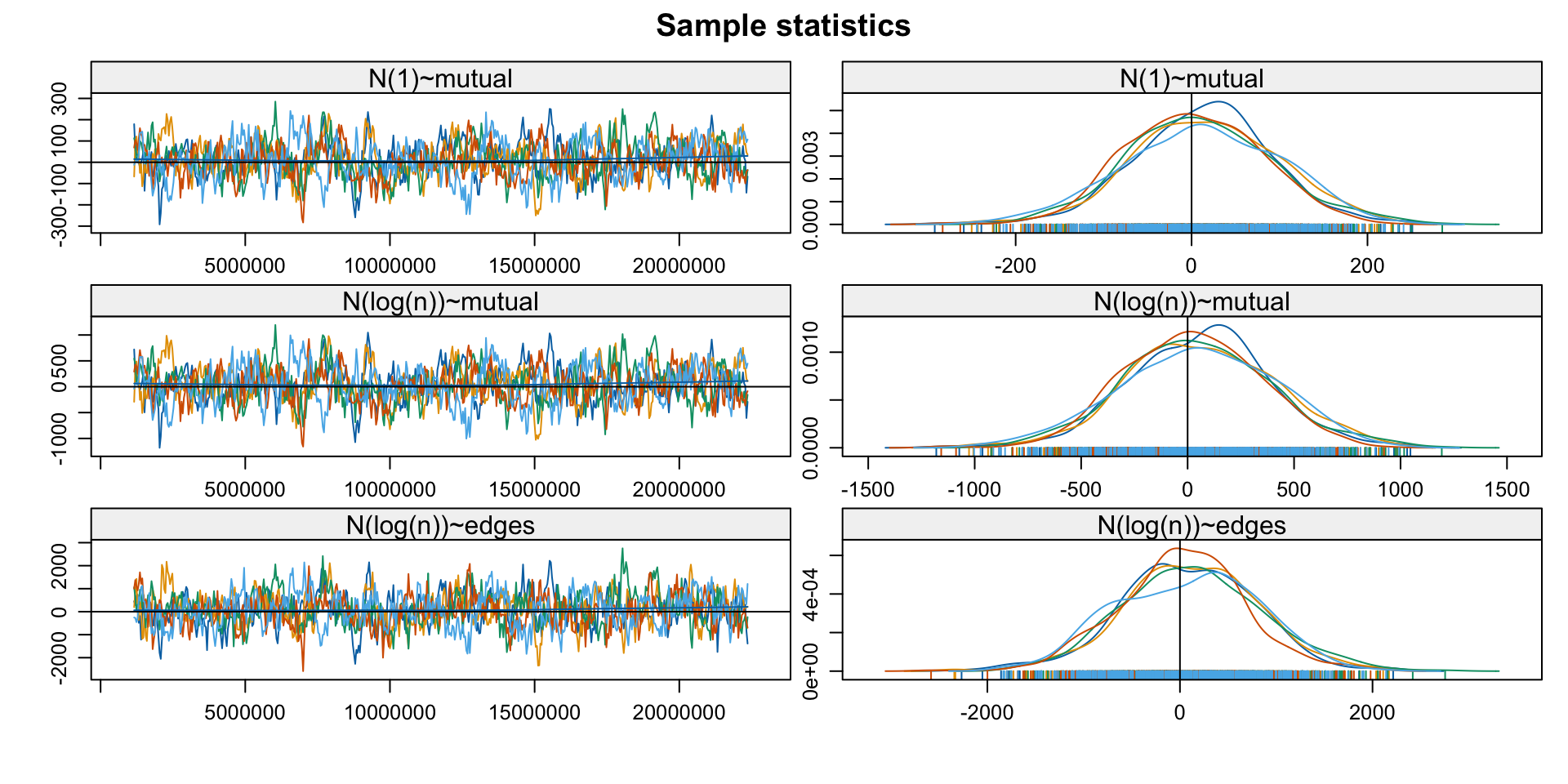
Note: MCMC diagnostics shown here are from the last round of
  simulation, prior to computation of final parameter estimates.
  Because the final estimates are refinements of those used for this
  simulation run, these diagnostics may understate model performance.
  To directly assess the performance of the final model on in-model
  statistics, please use the GOF command: gof(ergmFitObject,
  GOF=~model).
3. Diagnose: GoF
Code
simulated <-  mapply(FUN = function(x) {
  tmp_x <- get_within_networks(x, x%v%"block")
  summary(tmp_x ~transitiveties + triangle + edges + mutual)
}, x = sim_networks,
SIMPLIFY = FALSE)
simulated <- do.call(rbind, simulated)
state_twitter_block <- get_within_networks(state_twitter, twitter_res$block)
observed_statistics <- summary(state_twitter_block ~ transitiveties + triangle + edges + mutual)
plot(density(simulated[,1]), xlab = "Transitivities", ylab = "Density", main = "")
abline(v = observed_statistics[1], col = "red")
3. Diagnose: GoF
- Plot the goodness-of-fit statistics


